The United Nations backed the new Equal Earth world map. The Mercator projection, created in 1569, is just one visual representation of the landmasses designed to facilitate sea navigation.
The Mercator projection is also a PITA for radio signal propagation analyses.
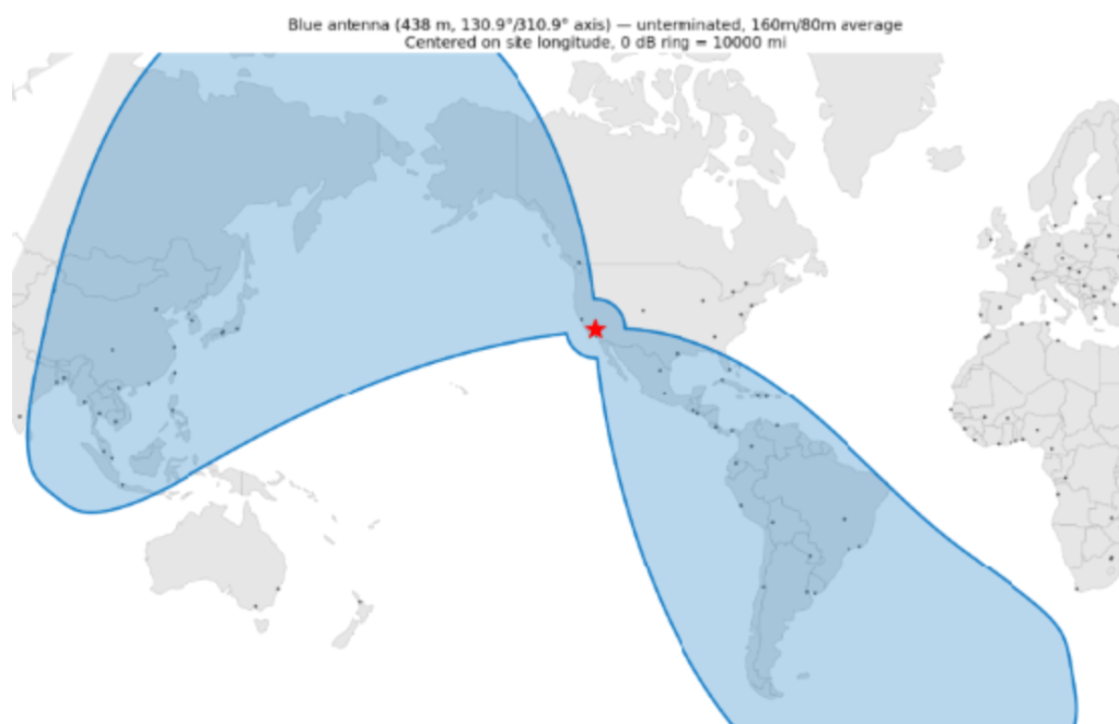
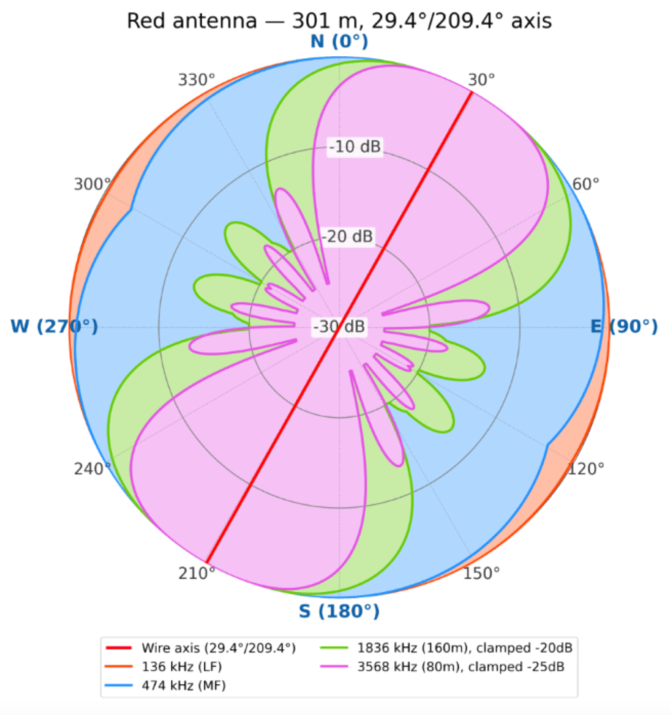
We have four Beverage antennas for long-wave, low-frequency bands. To have an idea of which direction the antennas are pointing, a simplified but “somewhat representative” lobe plot of the blue antenna on a Mercator projection map looks like this:
While correct, it sits askew in the human brain — the wire can’t seem to cover a “narrow” slit of South America while engulfing everything from western Canada to Asiatic Russia, Japan, much of China, and Indonesia.
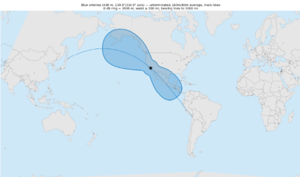
A Mercator projection is already an unfulfilling attempt to flatten a sphere onto a rectangular sheet; A little fudging of the pattern to aid comprehension was fair game. It resulted in this plot:
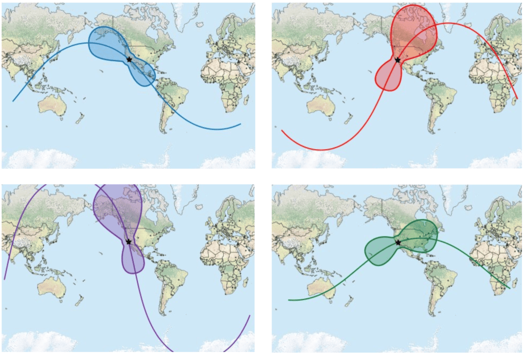
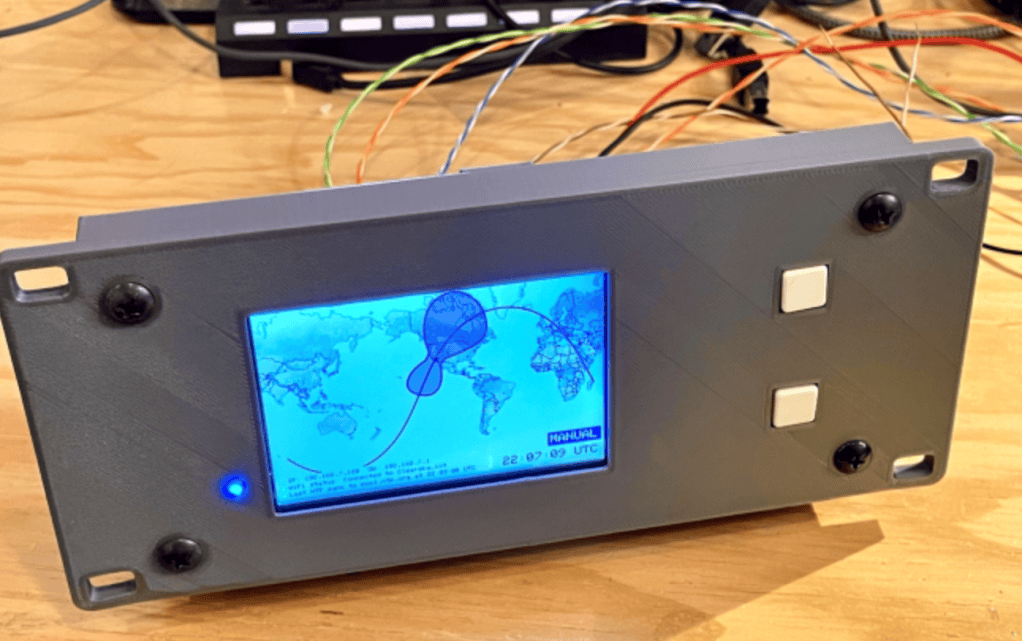
Besides being easier on the brain, it also aids glanceability on our custom Beverage antenna switching device, which rotates between four antennas on a 3.5-inch screen. Here’s how the four maps look with a bit of a “cartoon” treatment:
Tweaking maps for specific purposes, from navigation to readability and data analytics, is nothing new. For our setup, the improved glanceability helps us ingest more information quickly and identify relevant data much more easily.
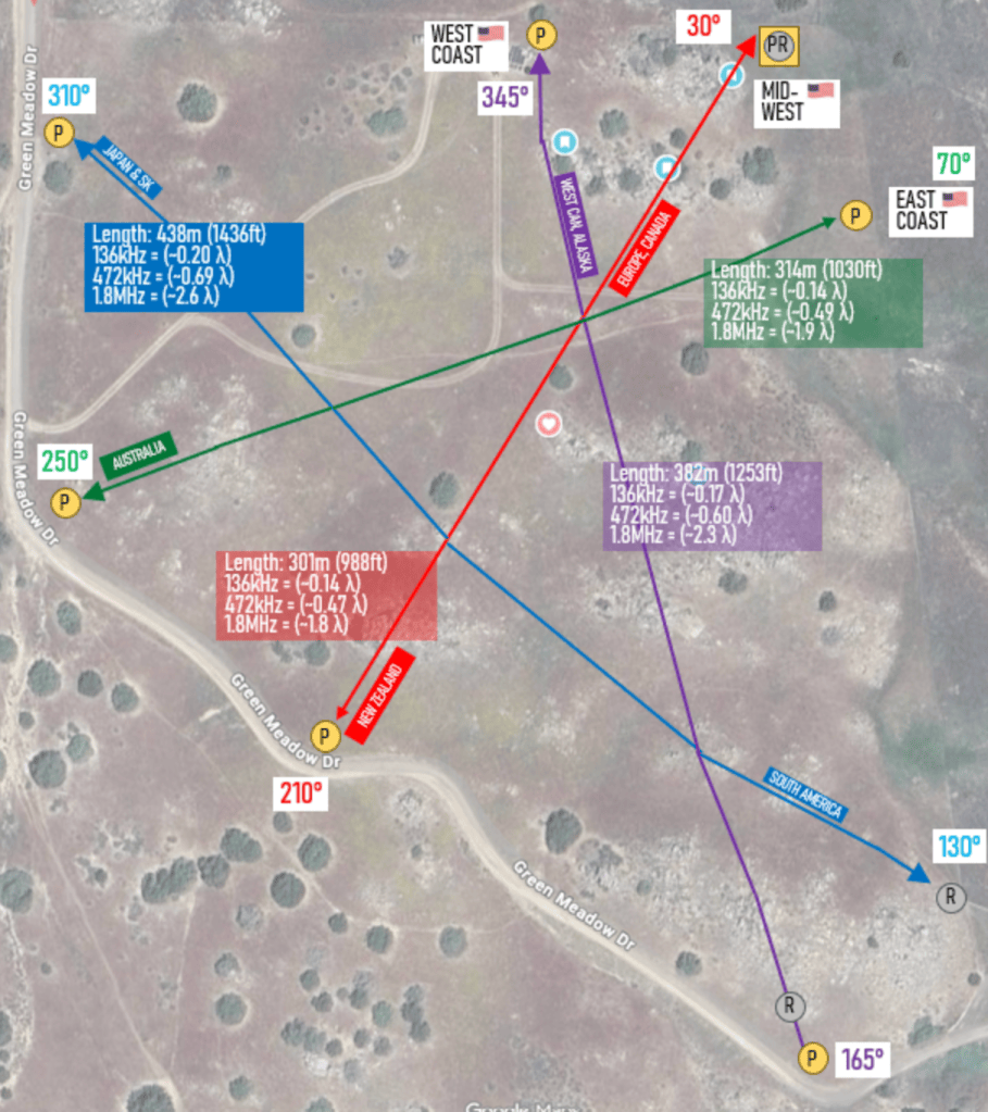
At Clearsky, we have longwire Beverage-style antennas at 45 degrees for longwave and lower shortwave work. We typically leave them unterminated, so they receive equally well in either “endfire” direction.
Since the radiation pattern is dependent on the length of the antenna relative to the frequency of interest, a simplified plot of the directional response of the “red” Beverage on the 2200 meter band, the 630 meter band, the 160 meter band, and the 80 meter band roughly looks like the following when plotted on a linearly concentric-in-dB chart.
To manage switching between these antennas, we designed and built a Beverage antenna switching device. It has automatic and manual modes, connects to our IoT WiFi, pulls UTC time from an ntp.org server, and rotates between four antennas at two-minute intervals to coincide with WSPR transmissions.
It is built around a 3.5-inch TFT display attached to an ESP32-Wroom microcontroller system, wired to a relay board, and uses an I2C expander to read the two “user interface” buttons and drive four double-pole, double-throw relays.
For receiving, we wired the entire station with 100-ohm differential CAT-6 cable. Impedance-control-wise, that system plays well with DPDT relays. (If that were to matter, but it doesn’t at the frequencies of interest.)
The case is 3D printed, 8 inches wide, and will go into a rackmount system. We have 8-inch, 10-inch, and 19-inch racks, all with standard 1U vertical offsets.
The top button allows for manual cycling between the four antennas. Pushing the top button activates the selected antenna indefinitely. Tapping the lower button switches the unit into automatic, 120-second rotation mode.
Our site features four Beverage antennas, each running 500+ feet, positioned at 45-degree intersections to cover the full compass rose. That’s a lot of wire, a lot of real estate, and a nontrivial cable run back to the lab from every corner of our 20-acre site.
The signal needs some help to survive that drop, so we’re building a dedicated amplifier from scratch using only in-stock parts, since receiving parts at a remote site like ours could take weeks. For example, we stockpiled Fair-Rite Mix 75 toroids from Digi-Key several months ago specifically because we knew this project was coming.
Why a custom amplifier?
Off-the-shelf preamps exist, but they’re optimized for narrower use cases. We need to cover the full span from VLF up through 160m and optionally 80m, from 25 kHz to 3.5 MHz.
That range creates a specific design tension: at the lower frequencies, the Beverage is electrically short relative to the wavelength, so it behaves more like a voltage source than a current source. At higher frequencies, it’s properly in Beverage mode — a traveling-wave antenna with a characteristic impedance around 400 ohms when terminated.
We landed on 2 kΩ as the input impedance, roughly 5x the terminated Beverage impedance, to achieve a reasonable compromise between the two regimes. Since the antenna is atmospheric noise-limited, we don’t sacrifice signal-to-noise ratio by going high-Z.
A few hours in LTSpice
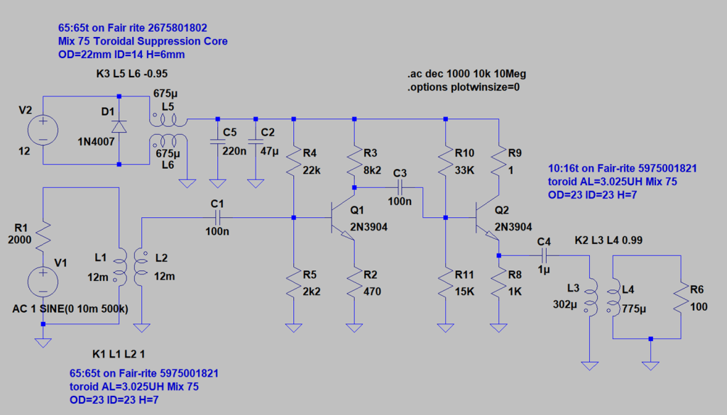
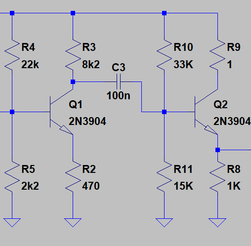
With those constraints locked in, we fired up LTSpice. A couple of hours later, we had a design: a two-stage BJT amplifier with an emitter follower (Q1) feeding a common-emitter gain stage (Q2), both biased at conservative operating points (1 mA and 3 mA collector current).
Transistor selection isn’t critical since noise performance here is dominated by the atmospheric environment, rather than the device — BC547, 2N3904, and 2N2222 will all work. We may compare them anyway out of curiosity.
A note on the simulation grounds
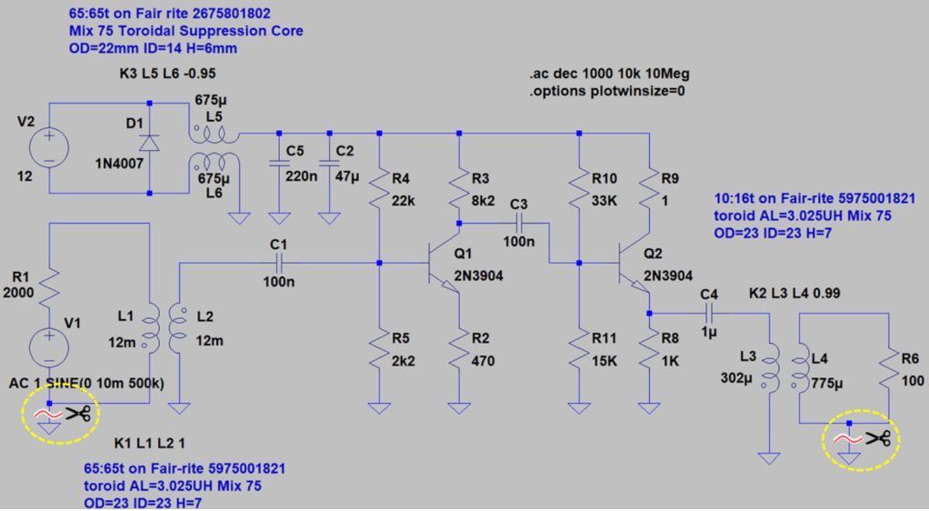
In one distinct way, the simulation doesn’t represent the physical build: the power supply, input signal, and output signal sections are intentionally not tied to a common ground. Connecting them would open the door to ground loop currents that would foul the signals we’re after. It would also defeat part of the purpose of the transformers (L1/L2, L3/L4, and L5/L6): the first two allow different ground domains to float relative to one another, denying undesirable ground currents a path.
That floating behavior makes LTSpice unhappy. Without a common reference, potential differences are limited only by stray capacitance and other parasitics — and we’re not even confident the model captures those accurately. The result is the simulator cheerfully reporting femtoamps and gigavolts, which contributes nothing to comprehension. Anyone who’s spent time in a physics simulator knows the phenomenon. So we tied them to a common potential for the sim, and the scissors symbols on the schematic mark where those connections get cut in the real build.
Power supply: keeping the junk out
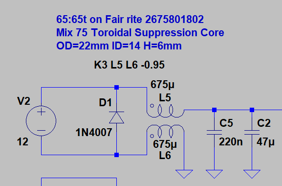
Power arrives via a second twisted pair on the same CAT-6 run at 26V, regulated down to 12V (not shown in the schematic). Right after the regulator is a common-mode choke that intercepts RFI and inverter line noise before it gets anywhere near the amplifier.
That choke is 65 turns wound bifilarly on a Fair-Rite 2675801802 Mix 75 suppression core. The datasheet doesn’t specify AL directly, but back-solving gives us approximately 3,000 nH/T², which works out to about 12.7 mH of inductance. At 25 kHz, that’s 2 kΩ of impedance. At 136 kHz, nearly 11 kΩ, and at 472 kHz, 38 kΩ. The choke pairs with a ceramic/electrolytic cap combination to form a low-pass filter that bounces common-mode noise back where it came from.
Input transformer: isolation with a DC path
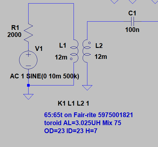
The input stage uses a 1:1 isolation transformer (un-un) rather than a direct connection to minimize static. The air at our site is extremely dry, and static buildup is an operational hazard. For instance, we’ve observed disconnected coax cables arcing over in the lab with nothing attached. The transformer provides isolation while still giving the antenna a DC path to ground.
We use the same core material, 65 turns bifilar again, this time on a Fair-Rite 5975001821 (AL = 3,025 nH/T²). Here’s the math to set the −3 dB point at 25 kHz:
L = 2000 / (2π × 25,000) = 12.7 mH
N = √(12,700,000 / 3025) ≈ 65 turns
The inter-turn capacitance isn’t a concern because even a generous estimate of 500 pF gives a reactance of 12.7 MΩ at 25 kHz.
The upper frequency limit is set by leakage inductance. For a well-wound bifilar toroid, leakage is typically 0.5–2% of magnetizing inductance:
L_magnetizing (65t) = 65² × 3,025 nH = 12.8 mH
L_leakage ≈ 1% = 128 µH
f_upper = 2000 / (2π × 128 µH) = 2.49 MHz
That puts us right at the 160m band target. The catch is that achieving 1% leakage requires tight bifilar winding. Sloppy technique would push leakage to 3–5%, dragging the f_upper down to 800 kHz–1.2 MHz and visibly costing us at the top of the band.
Amplifier stage
The two-transistor topology is straightforward. Q1 is an emitter follower with high input impedance and unity voltage gain. It drives Q2, a common-emitter stage with the actual power gain. Operating points are conservative and stable.
Output transformer: matching the cable
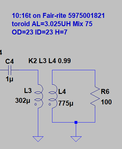
CAT-6 has a characteristic impedance of 100 Ω. The amplifier output impedance is about 40 Ω. The output transformer bridges that gap.
We use the same Fair-Rite 5975001821 core, AL = 3,025 nH/T². The impedance ratio is 2.5:1 (100 Ω to 40 Ω), which gives a turns ratio of √2.5 ≈ 1.58. In practice:
At 136 kHz: XL = 258 Ω — about 6.4× source impedance, ~1 dB rolloff ✓
At 25 kHz: XL = 47.5 Ω — ~1.2× source impedance, ~7 dB rolloff ✓ (within budget)
At 2 MHz: XL = 3.8 kΩ — well above source impedance, flat ✓
The 7 dB rolloff at 25 kHz looks steep on paper, but signals at the very low end are strong. We’re comfortable with it.
Simulated performance
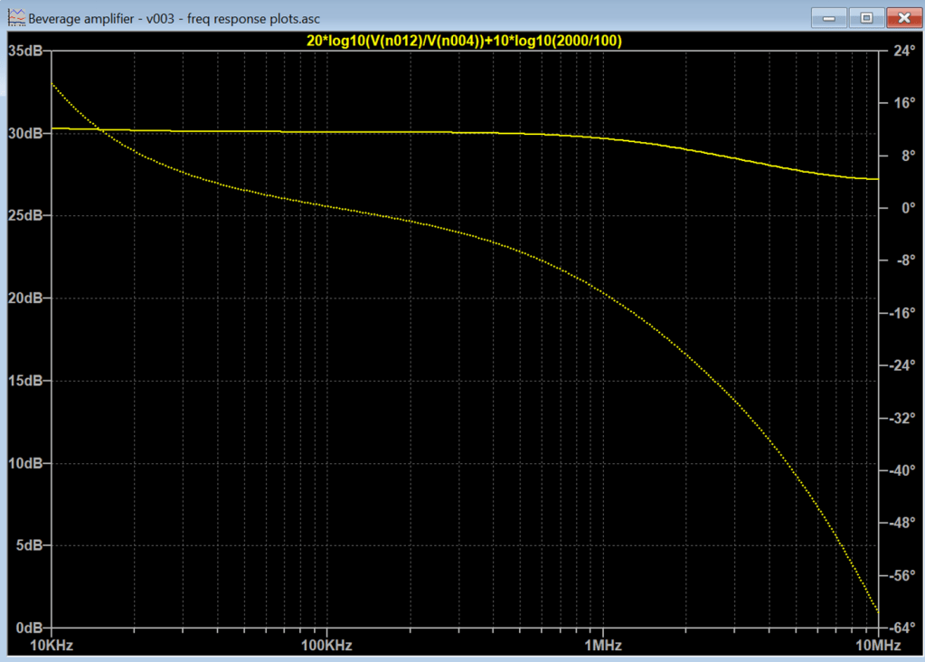
The assembled simulation shows approximately 30 dB power gain, flat from VLF to 1 MHz, dropping to 29 dB at 1.8 MHz and 28 dB at 3.5 MHz.
The Mt. Wilson stress test
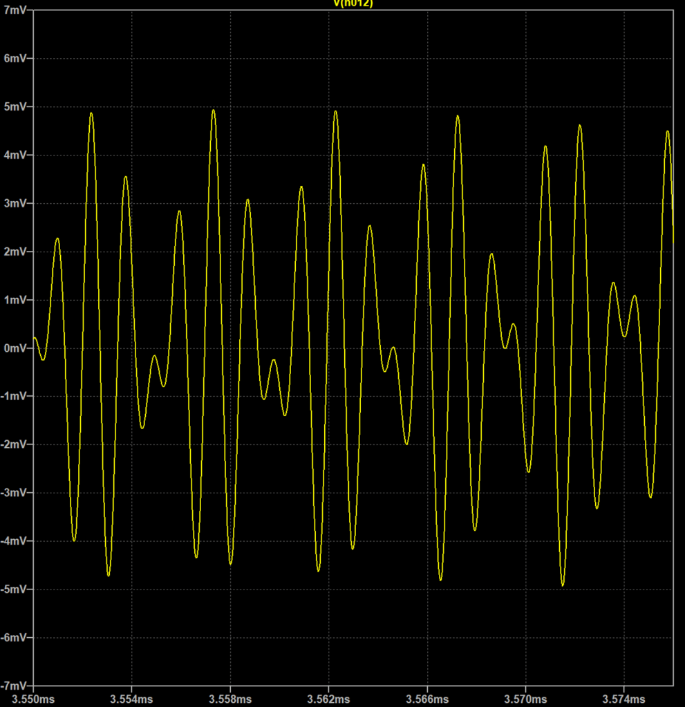
The AM broadcast cluster on Mt. Wilson near Los Angeles, roughly 80 miles south, is the obvious stress case. Two stations, 600 kHz and 810 kHz, were injected at a pessimistic 1 mV each (a conservative assumption). It looks messy in the time domain.
Intermodulation products are 70 dBc down in the frequency domain. We’ll take it.
Next step: build the thing
The simulation is solid, and the parts are on hand. Time to wind some toroids. We’ll report back.
Our container lab sits on decomposed granite, and the ground is absolutely terrible for driving ground rods. When we needed a serious RF ground for our 630m band work, the conventional answer — an 8-foot copper-clad rod hammered vertically into the earth — wasn’t going to happen. The rock laughs at you.
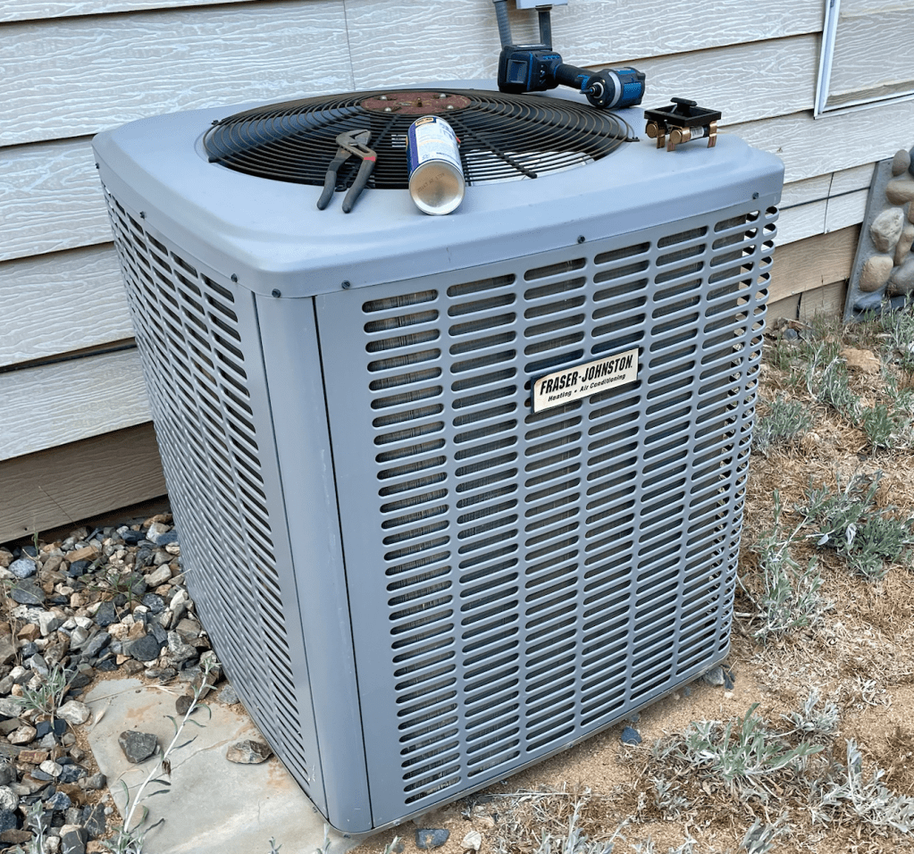
So we stripped a dead air conditioner instead.
Taking inspiration from the NEC
Our existing safety ground works fine at 60Hz. However, at LF/MF frequencies, its inductance makes it useless as an RF reference. We need a separate, dedicated low-inductance, low-impedance path to earth for the RF system.
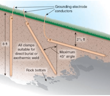
Which brings us to a useful detail in the National Electric Code Section 250.53(G). It’s intended for safety grounding, but the physics doesn’t care. It states that if bedrock or other impediments prevent driving a standard 8-foot rod vertically (or at up to 45 degrees), it’s permissible to bury it horizontally at a minimum depth of 30 inches.
This gives us an out for our predicament. How? You see possibilities once you understand why horizontal burial works just as well as vertical. Let’s dig in.
Orientation barely matters, while surface area is everything
The key insight lies in the geometry of how resistance works in soil. If you model the earth around a buried electrode as concentric hemispherical shells, the innermost shells, i.e., the soil immediately surrounding the electrode, dominate the total resistance. Beyond a few multiples of the electrode’s largest dimension, additional soil contributes almost nothing.
The resistance of each shell of thickness (dr) at radius (r):
dR = (ρ · dr) / (2πr²)
Integrating from the electrode surface radius (a) to infinity:
R = ρ / (2πa)
Here’s the practical implication: what matters is the effective radius a, which is determined by the electrode’s surface area in contact with the soil, not whether it’s pointing up or sideways. A horizontal rod at 30 inches deep achieves soil contact of the same quality as a vertical one. Current just spreads outward horizontally instead of downward.
This is good news for anyone with bedrock close to the surface, and great news if you happen to have access to something with a lot more surface area than a rod.
Enter the dead air conditioner
When a neighbor was upgrading her HVAC system, we offered to haul away the old Fraser-Johnston condenser unit. We saved her the disposal headache and got a potentially useful hunk of metal.
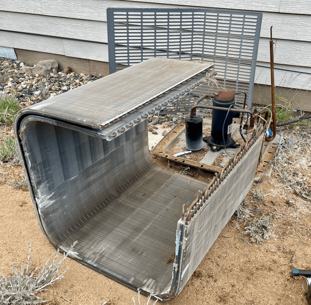
Once we stripped it down, we found RF gold: a massive condenser coil. It’s a large, U-shaped assembly of copper tubing bonded to aluminum fins. Unrolled flat, it measures roughly 1.5 × 5 meters, providing about 7.5 square meters of copper-bonded surface area.
Compare that to a standard 8-foot × 5/8-inch ground rod, which has an effective surface area of about 0.04 m². Let’s run the numbers for decomposed granite soil (resistivity ρ ≈ 10,000 Ω·m, a reasonable estimate for dry granite):
Electrode
Effective radius
Resistance to remote earth
Standard 8 ft rod
~0.008 m
~200,000 Ω
Copper/aluminum plate, 1.5 × 5 m
~1.55 m
~1,000 Ω
That’s roughly a 200:1 improvement over a standard rod in our specific soil conditions.
A note on the oxidized copper: the coil has surface oxidation, as you’d expect from years of outdoor service. Copper oxide remains sufficiently conductive at these frequencies, so it doesn’t meaningfully affect performance.
One more wrinkle: skin depth in soil
Soil has a skin depth just like a conductor, and the depth at which RF current density falls to 1/e of its surface value:
δ = √(ρ / (πfμ₀))
Where ρ is soil resistivity, f is frequency, and μ₀ = 4π × 10⁻⁷ H/m.
For our decomposed granite at 472 kHz, that works out to roughly 15 meters.
The practical implication is that at our primary operating frequency, the current penetrates deeply enough that the burial depth of our electrode matters much less than its lateral extent. We’re well within the quasi-static near-field regime: the plate’s 5-meter dimension is about λ/300 at 472 kHz, which means we don’t have to worry about resonance or standing-wave effects.
Into the ground
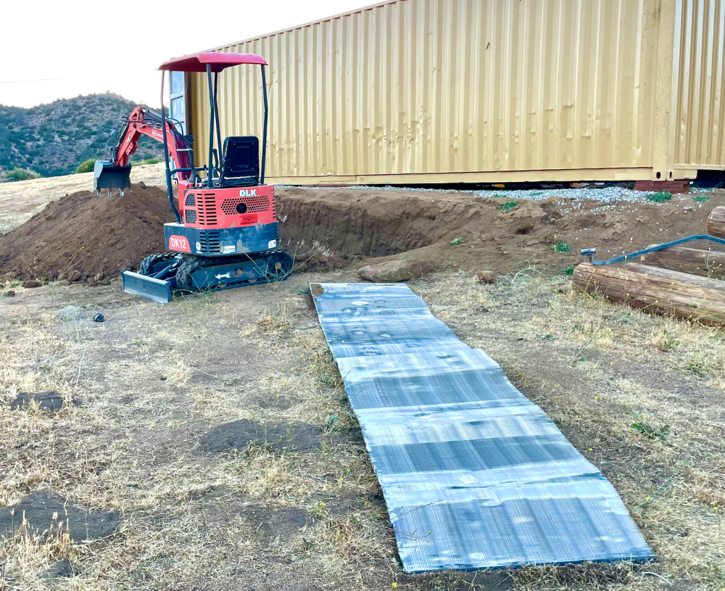
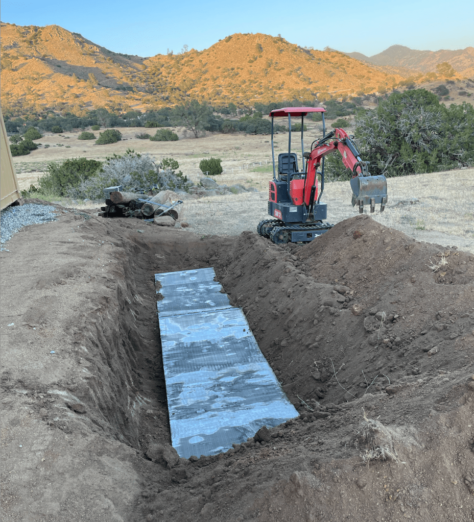
We dug a trench (as deep as humanly possible without involving dynamites) next to the container lab using a mini excavator, laid the coil flat, and buried it at approximately 2 feet below grade. We may add more backfill on top, which would only improve performance because more soil mass above the plate means better coupling to the surrounding earth.
As a natural Faraday cage, the container lab is the most suitable location for this ground reference. Bonding the plate to the RF entry point at the lab keeps the connection path short and low-inductance, which is exactly what we need.
The key to low inductance is to keep the connection length between the grounding plate and the container lab as short as possible. We have about 4’ to cover, which is far closer than most people can achieve. We also use two AWG6 conductors (code only requires one) to further reduce inductance.
Results, not paperwork
A purpose-built ground system for a research site like ours with engineered plates, burial contractors, and the works would require a budget line, a procurement process, and probably at least a few months of waiting. We did this on a Tuesday with our mini excavator and a condenser coil headed for the scrap pile.
The physics says it should outperform a standard rod in our soil by roughly two orders of magnitude. We’ll validate that against measured ground resistance once the bond is complete. But the modeling is solid, the plate is in the ground, and the price was right.
We build minimum viable infrastructure grounded in actual physics to test theories and validate ideas — enabling researchers to deploy experiments before anyone’s written a scope of work or grant proposal.
Ready to run your own budget-friendly RF experiment? Drop us a line.
We believe in dark data. And we’re creating more of it.
That probably sounds backwards, so let us explain.
What is dark data, anyway?
In the data world, “dark data” refers to information that gets collected but never analyzed, such as logs sitting on a server somewhere, sensor readings that feed nothing, and archives nobody has touched in years. It’s there, but no one can access the insights.
Consider astronomy: researchers have been discovering new celestial objects by analyzing telescope images through modern tools. The data existed, but the tools to interrogate it hadn’t caught up yet. When they did, our understanding of the sky evolved.
Radio is heading in a similar direction. Decades of RF experimentation, propagation logging, and signal data are sitting in archives. Newer machine learning tools — not the chatbot kind, the pattern-recognition-in-large-datasets kind — are getting good enough to find structure in that noise.
The question is whether there’s enough data to work with, and whether it covers the right parts of the spectrum. For most of the spectrum, the answer is yes. For the long waves, not so much.
A century-old detour
Radio started on the long waves. The earliest wireless telegraphy operated at wavelengths measured in kilometers, and for a brief period, that’s where all the action was.
Then, technology caught up, and everyone moved on to HF, VHF, UHF, and microwave. Each step up the frequency ladder brought more practical antennas, more bandwidth, and better noise floors. Long waves became a curiosity, and eventually, frequencies most engineers actively avoid.
That shift made sense. If you’re trying to stream data or run a cellular network, there is nothing useful about a wavelength you can’t fit in a city block.
But “not useful for communications” doesn’t mean “scientifically insignificant.”
What long waves can do that nothing else can
Low frequencies have unique properties. Substances that stop a microwave dead, such as oil, rock, and water, are partially transparent to a long wave. That makes subterranean imaging a real possibility yet to be explored.
The atmospheric behavior is different, too. Long-wave propagation is sensitive to conditions in the ionosphere and lower atmosphere in ways that HF and above simply aren’t. Long-wave data offer valuable insights to researchers studying pre-seismic electromagnetic anomalies, atmospheric conductivity shifts, space weather signatures, and more.
The problem is that the data barely exists. The petabytes of RF data humanity generates every day come from medium-wave and up (e.g., AM radio, cellular, WiFi, and 5G). Long-wave coverage is thin by comparison, mostly because working in that part of the spectrum is genuinely challenging.
Why long waves are hard
Operating below 500 kHz is an exercise in fighting physics on multiple fronts simultaneously.
Radiation resistance in the long waves is measured in milliohms. Your antenna is working against an impedance that makes a short circuit look like a good deal. Atmospheric noise is severe. Everything connected to a power outlet contributes to interference. Meanwhile, current simulation software doesn’t handle propagation modeling in complex terrain well.
Then, there’s the space problem. A quarter-wave antenna at 472 kHz is about 158 meters tall. Nobody’s building that in their backyard. Even a practical compromise like a loaded vertical or an inverted L demands a large property, a serious ground-radial system, and ideally some elevation. An acre of ground radials barely gets you started.
Next, we must consider location. Long-wave signals are extraordinarily sensitive to interference from the power grid, switching regulators, and nearby electronics. Suburban or semi-rural sites with neighbors, grid noise, and cellular infrastructure are non-starters. You need genuine RF silence, which means distance from populated areas and natural terrain shielding.
That combination of acreage, RF isolation, and terrain that doesn’t actively destroy propagation is rare. Most people who want to experiment in this part of the spectrum don’t have access to it.
We do. Our 20-acre site in Kern County sits at 3,500 feet in a natural bowl surrounded by mountains. There’s no cell service. Broadcast intrusion is minimal. The terrain provides shielding that can’t be replicated with filters. The noise floor is low enough that subtle, slow-moving effects that take weeks of continuous monitoring to become visible actually show up in the data.
What we’re doing with the data
Our site features a mix of open terrain and canyon geometry that creates unusual propagation conditions. We run a multi-antenna setup across several bands, including 630m (472 kHz), with ongoing experiments on ground-wave behavior, atmospheric correlation, and signal propagation in challenging environments.
Before starting ClearSkyRF, I spent decades in battery analytics, machine learning, and high-performance RF design from UHF to Ku-band before landing on this particular obsession. The through-line is the same in all of it: large datasets plus novel analysis tools reveal things that weren’t visible before.
We think the long waves have secrets. We’re here to find out.
We have serious antenna plans. The good news is that executing them doesn’t necessarily demand a serious budget. Instead, it requires knowing where to look and the willingness to put in some elbow grease.
Over the past couple of years, we’ve been building a stash of dishes, poles, and towers that most research facilities would have to write a procurement justification, wait months for funding, and then more months for execution. Here’s how we bootstrap the whole thing.
MVPs find the right direction
We don’t wait until we have the “right” setup before we start learning. We stand something up, learn from it, and refine after proving that we’re heading in the right direction. Our gear stash exists to make these cycles low-cost and fast.
Case in point: our current antenna field includes everything from a fan dipole strung over a canyon to a full-wave 630m loop — the seed of what will eventually become our Giga Loop, a receive antenna covering over 15 acres of the property.
None of that happened by waiting for the perfect conditions or equipment. We build the minimum viable experiments, learn from them, and iterate from there. Let’s take a closer look at our gear stash and the story behind the pieces.
Free Ku-band dishes from neighbors
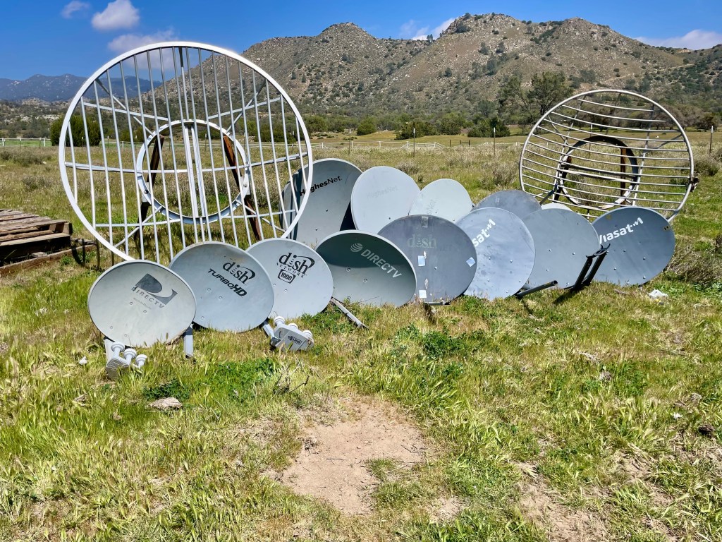
Rural neighbors upgrading to Starlink have one problem: what to do with the old HughesNet and Viasat hardware bolted to their roof or fence post? We solve that problem for them by taking the dish off their hands. Everyone wins.
The result is a growing collection of consumer satellite dishes, roughly 18 to 30 inches in diameter, from DIRECTV, Dish Network, HughesNet, Viasat, etc.
Applying Ku-band dishes to RF research
The smallest dishes (e.g., DIRECTV and Dish Network) are the least useful for us. With some exceptions, such as possible amateur use at 24GHz, the Ku- and Ka-band dishes aren’t effective parabolic reflectors. They don’t gather enough signal because they’re too small relative to the wavelengths we work with, and smaller dishes collect less signal anyway.
Why keep them in our mix? They weigh less and are physically easier to work with. They catch less wind and are sturdier. These characteristics make them prime material for testing new motorized azimuth/elevation tracking systems: we’ll know the target satellites’ positions and auto-calibrate our tracking systems by finding the maximum signal strength for a satellite.
Moreover, we can use universal feed mounts to attach X-band feeders to these Ka-band dishes. That doesn’t seem to make sense, as the gain will be low and the signal will be out of focus. However, that “weak, wide, and fuzzy” field of view will be beneficial when we take numerous repeated “quick whole sky” surveys, as smaller dishes can move faster and scan wider swaths of sky per streak.
Of course, there’s no free lunch. We pay the price in lower signal strength and less precision. However, the many wide-field-of-view low-res scans can give us insights that fewer, narrower beam-width high-res scans cannot. It’s like using a wide-angle lens to take high-ISO pictures to identify where to look before strapping on a long lens and taking a long-exposure photo for precision.
The hunt for giant C-band dishes
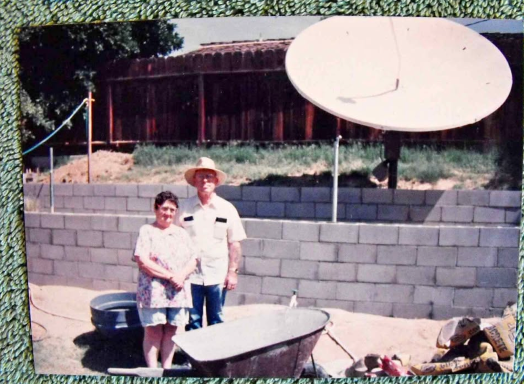
Before small dishes took over in the mid-90s, rural America ran on large C-band parabolic dishes — typically 8 to 12 feet across. Most of them are still out there, sitting in fields and backyards, inherited by people who have no idea what to do with them and no desire to move them.
We scored a couple of these from folks in our community and one from Facebook Marketplace. Even the transfer station attendant knows to keep a lookout for us.
Applying giant C-band dishes to RF research
A 10-foot dish is 20 times the longest wavelength, big enough to provide meaningful gain for S-band, such as tracking space missions (e.g., Artemis 2 operated on the 2.2 GHz band). Assuming a high surface precision, these dishes can work up to any microwave frequency we want to play with. In fact, the higher the frequency, the higher the gain and the narrower the bandwidth.
However, pivoting that behemoth around isn’t a zippy affair. It’s also hard to do that with high precision. As such, we use the smallest dishes to meet a study’s requirements, not the 10-footer for everything.
And yes, we’ll try moonbounce on the 13cm, 9cm, 5cm, and 3cm bands.
Our telephone pole pipeline
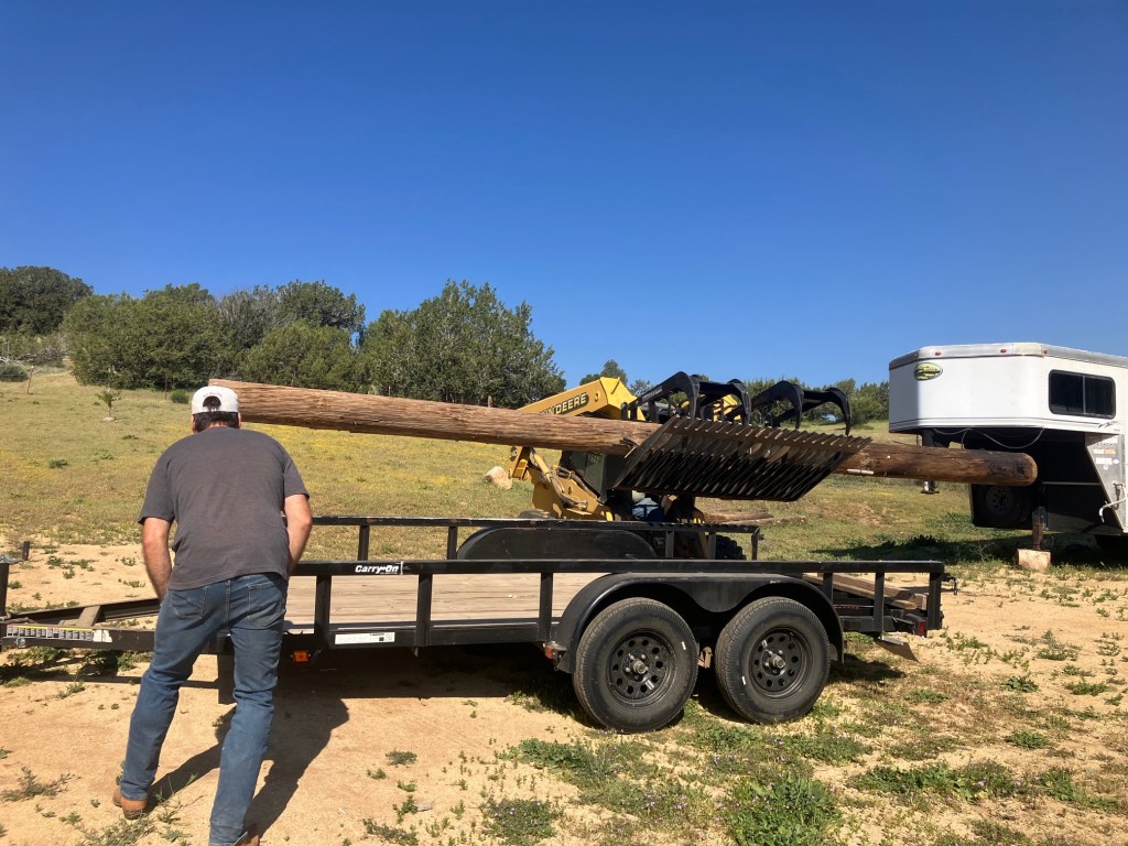
Old utility poles are a rural constant: properties accumulate them over decades, and nobody wants the hassle of removal or hiring someone to truck them out. We put the word out that we’re looking for phone poles, and people just say, “Come get ‘em!” We score pieces up to 27 feet tall — essentially a free antenna mast, already seasoned by years of outdoor service.
These are the workhorses behind our Beverage antenna wire support: quick to deploy, cheap to source, and sturdy enough for long wire runs across our 20-acre site. When an antenna design calls for spans stretching 1,500 feet across the site, not having to buy masts makes a real difference to the budget.
Beverage antennas don’t need to be high off the ground; just elevated enough so that roaming cattle and other animals don’t ruin them (fun fact: we’re in an open range area!) The stubby poles are great for this purpose and can also provide a sturdy base for temporary small masts. For example, we can strap a 30-foot mast to these poles, as long as the winds are under 70 mph.
Will drive 4 hours for antenna towers
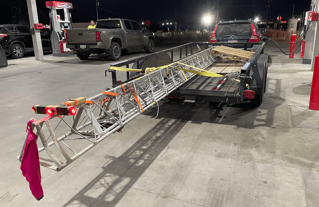
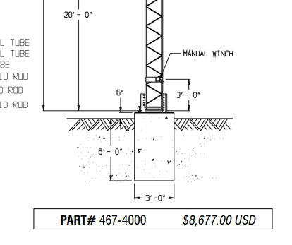
Telephone poles do the job, but antenna towers do it better. Yet, any ham operator who’s priced out new tower sections knows they’re a serious line item. For example, we recently scored a 67-footer that’s equivalent to the Tashjian WT-67 with an $8,677 price tag in its basic form, excluding transportation costs.
The good news is that used towers are a different story if you know where to look. Some people might have inherited them when they purchased a property. Some have to part with them because HOAs really don’t like them.
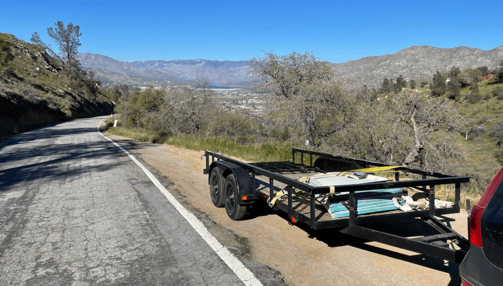
We scout Facebook Marketplace for these towers across rural communities and make the long drive to get them, once a 4-hour one-way with a 14-foot trailer.
These sections are modular, allowing us to dial in the exact height required. They’re also lighter and easier to maneuver on-site thanks to built-in mounting provisions. Of course, not all of them are in ready-to-deploy shape. Some repair work and elbow grease are required before we can put them into service.
Using antenna towers in our RF research
Conventionally, these towers are used to support rigid antennas. Most commercial installations have fixed antennas, while most amateurs want rotatable beams. We’ll do neither of those and use the towers primarily for supporting wire antennas that must be high off the ground to work well.
We plan to use our two tallest towers (54 and 67 feet), which are easy to crank up and down, as agile bases for long wire antenna experiments. Others, like the fixed 35-foot Rohn 25, will be used as elevating structures to augment the effects of the canyons in our fixed installations.
Results, not red tapes
Building this gear stash isn’t glamorous. It involves Facebook treasure hunts, trailer runs on steep dirt roads, and a lot of quality time with ratchet straps. But the upfront effort means that when an experiment calls for a 10-foot dish or a 40-foot mast, we’re not waiting on a purchase order — we’re already setting it up.
There’s a certain humbling quality to working at 472kHz. You pull up the math, realize a proper half-wave vertical would need to be over 300 meters tall, and then you have a moment. A long moment.
Then, you get creative.
Let’s dive into how we approached building a transmit antenna for the 630m band at our Kern County site. This post explains why we selected the inverted L configuration, how we leveraged the landscape to avoid a massive tower, what our simulations predict, and what we hope to learn once the antenna is operational.
472kHz is a pain in the neck but worth the trouble
At 472kHz, your antenna wants to be enormous. A half wavelength is around 315 meters — taller than the Eiffel Tower. So a “proper” full-size vertical is off the table for us mere mortals outside the broadcast engineering world.
But setting up the antenna isn’t just for the game.
The 630m band is relatively uncrowded and, compared to HF bands, surprisingly understudied, partly due to antenna size limitations and partly due to site availability.
Most existing research on LF and MF propagation comes from flat, low-elevation sites or coastal plains, where soil conductivity is high, well-characterized, and relatively uniform. Our site is none of those. At 3,500 feet above sea level in the Sierra foothills of Kern County, it sits in a natural RF-quiet bowl surrounded by mountains. It features rocky terrain, a known aquifer below, and almost no local interference.
That combination of elevation, geology, and low-noise environment is rare. As a result, we generate propagation data that doesn’t exist anywhere else. But still, why go through the trouble?
At 630m, signal behavior is shaped simultaneously by soil conductivity, terrain geometry, and ionospheric D-layer conditions. We provide a clean baseline to untangle those contributions. Our unique site condition takes this antenna beyond a radio project to a data source for researchers who currently have to work around gaps in available datasets:
Geologists and hydrologists can access empirical data on how 630m ground-wave signals interact with rocky, mountainous terrain and aquifer-influenced soil when modeling subsurface features. The data is thin in this discipline.
Atmospheric and space-weather scientists studying D-layer behavior can gain long-term observations from RF-quiet sites. Most existing datasets come from coastal or urban-adjacent receivers with noisy baselines.
Earthquake researchers investigating pre-seismic electromagnetic patterns can access data from a geologically active site. We’re in a seismically active country with interesting geology and a noise floor that lets subtle signals surface.
We’ll return to the impact on scientists and researchers shortly. First, let’s look at how the antenna itself can be built — affordably and without years of permitting hurdles.
Leveraging our site’s unique characteristics with an inverted L antenna
An inverted L antenna is exactly what’s on the tin: a wire that goes up vertically, then bends horizontally. The vertical section does most of the radiating work. The horizontal top section primarily loads the antenna electrically, helping it reach resonance at a physically manageable length.
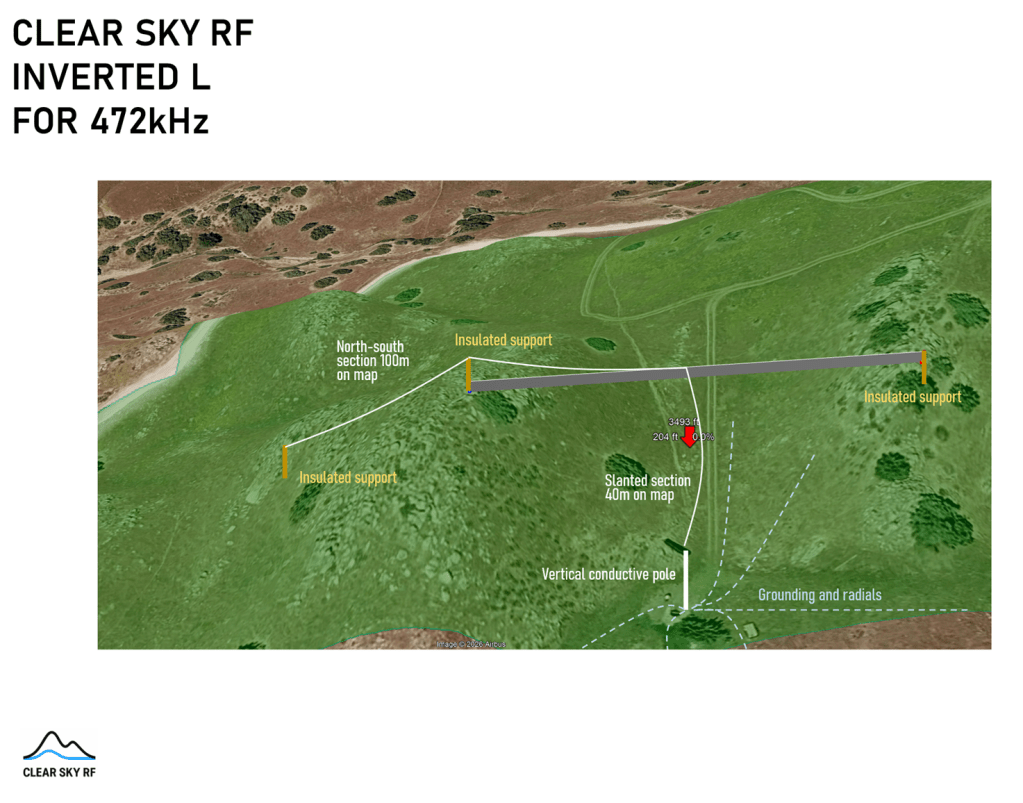
For our target frequency, we aim for a quarter wavelength, about 150 meters of wire. But how do we gain meaningful vertical height without a self-supporting tower? Solving this challenge is where our canyon earns its keep.
We plan to run a support wire from rim to rim across the canyon, with poles on both sides. The antenna’s vertical section rises from the feedpoint at ground level up to that support wire, where it makes a 90-degree turn and runs horizontally to one side, while the other end provides mechanical tension. The setup gives us usable height, sourced from existing terrain, and nature does the heavy lifting.
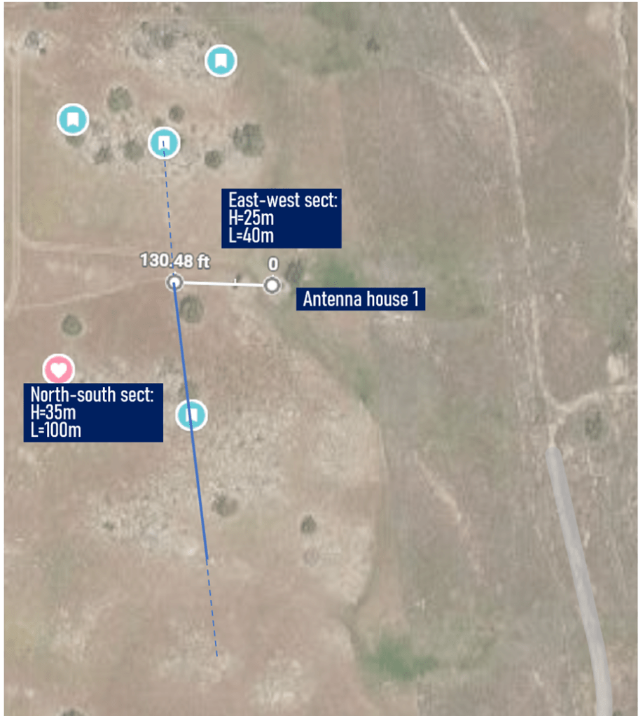
Site map
Here’s the full geometry breakdown:
North-south section: ~100m along the map, ~35m effective height
East-west section: ~40m along the map, ~25m height
Total wire length: ~150m (~quarter wavelength at 472kHz)
Antenna layout across the canyon
Another unique aspect of this build is that the antenna’s vertical section rises partly over solid terrain on the canyon rim, and partly suspended in open air over the canyon. While it’s possible to model an antenna over poor rocky terrain or in free space, current tools can’t cleanly model one that transitions between the two mid-wire.
We’re in greenfield territory.
A conventional approach to achieving what we’ve outlined would involve a 30-meter self-supporting tower, a concrete foundation, permit applications, and a significant budget. Such hurdles are exactly why we created ClearSkyRF to help accelerate RF research and use amateur radio as a tool to generate scientific, geologic, and atmospheric insights.
This is also how we challenge the “this is how things are done” mentality. We’re not here to build the definitive, fully optimized, write-it-up-for-IEEE antenna farm. We create something good enough to generate real-world data, learn from it fast, and decide where to dig deeper.
The unsung hero: a ground system that makes the difference
At low frequencies, a poor ground system will hurt your antenna efficiency more than almost any other design choice. The feedpoint of an inverted L antenna sits close to the ground, and its return currents flow through the ground. However, if that path is lossy, the power that should be radiating turns into heat instead.
Again, nature provides a solution: a clay soil layer with an aquifer underneath.
Our ground system consists of multiple grounding rods driven into the site’s clay soil section, combined with a radial wire network that spreads out from the feedpoint. We will build in the ability to connect or disconnect those radials independently, allowing us to run the antenna with and without them to directly measure the efficiency difference. Such a before-and-after comparison is more useful than any simulation, giving us real-world numbers for the actual soil condition.
For the baseline calculations, we use conservative soil parameters: a dielectric constant of around 13 and a conductivity of 0.0002 mS/m, typical for a rocky, mountainous terrain. In practice, we expect better numbers. The aquifer beneath our site will likely improve ground conductivity in ways that are difficult to predict precisely without direct measurement — understanding the difference is part of the experiment.
Simulation result with a pleasant surprise
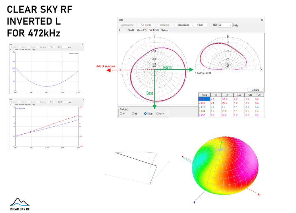
Before stringing a single wire, we modeled the antenna to check resonance, impedance, and radiation pattern. The numbers came back encouraging. At 472kHz, the model shows:
Impedance: R ≈ 6.8Ω, jX ≈ 3.5Ω — low resistance, as expected for a short antenna, which means a matching network will be needed between the feedpoint and standard 50Ω coax
SWR curve: Clean resonance across the 630m band
Gain: ~1.1 dBi — spectacular for this class of antenna
Simulation plots — SWR curve, impedance vs. frequency, radiation pattern
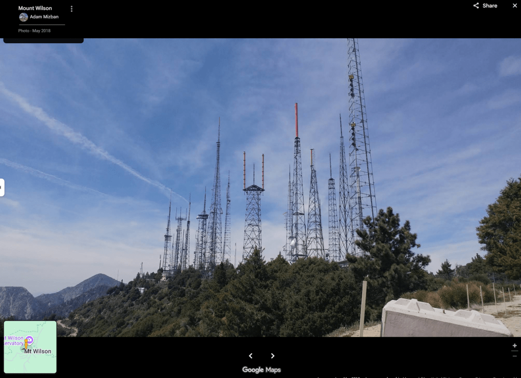
The radiation pattern also demonstrates a notable null of around 6dB of attenuation to the west. Follow that bearing, and you end up pointed at the antenna farm on Mount Wilson, north of Los Angeles. The dense cluster of high-power broadcast transmitters would otherwise contribute significant interference to any receiver in Southern California.
Mount Wilson tower farm
The null isn’t pure luck. The orientation and directionality of the horizontal top section determine how the pattern tilts and which direction the null goes. Run it north-to-south, and the null points one way. Flip it south-to-north, and the pattern flips with it.
We chose our orientation deliberately to put that null on Mount Wilson. In effect, we have some directional control over a 472kHz transmit antenna. As far as we know, no one else on the planet operates an electrically steerable antenna on the 630m band.
What this antenna will tell us
Once in the air, this antenna will be a transmit reference for experiments that are difficult to run anywhere else. These include:
Propagation characterization
By transmitting WSPR beacons on the 630m band and tracking their reception, we can build a propagation map based on our site’s characteristics, including elevation, terrain shielding, and soil, and compare the results against model predictions.
Ground-wave vs. sky-wave separation
At 472kHz, both propagation modes are active, and they behave differently over distance and time of day. Our low noise floor and known antenna geometry will allow us to distinguish them more cleanly than at a noisier site.
Soil and subsurface sensing
Ground-wave signal strength over distance is a proxy for soil conductivity. The gap between the assumed soil parameters and our measured antenna efficiency provides insights into what’s happening in the ground beneath us, including potential aquifer influence. The data will show us both ends of that equation, while the radial experiment will further sharpen the picture.
Atmospheric and space weather correlation
The 630m band is sensitive to D-layer ionospheric conditions, which respond to solar activity, geomagnetic storms, and some terrestrial weather patterns. Long-term continuous monitoring from a quiet, elevated site generates a unique baseline that makes anomalies visible and attributable.
Seismic monitoring potential
Pre-seismic EM anomalies in the LF and MF bands have been reported in the literature for decades, but the evidence remains contested — partly because clean, continuous datasets from geologically active, RF-quiet locations are rare. We’re in a position to contribute to that record in a way most sites can’t.
None of these is guaranteed. Some may turn out to be dead ends. That’s the point — the minimum viable experiment exists to explore possibilities without betting an entire facility on one hypothesis. And the inverted L antenna doesn’t have to do this alone.
Building a multi-antenna experiment
The inverted L is a transmit antenna. But what makes it genuinely useful as a research tool is how we pair it with other antennas.
We’re designing a regimen that alternates transmission and reception across other antenna systems on our site. The combination opens up comparisons that a single antenna can’t provide on its own.
On the receive side, we have two complementary tools. The Giga Loop is a full-wave 630m loop that will eventually encircle over 15 acres of the property. It picks up signals from all directions with a large effective aperture. Its size makes it unusually sensitive at these frequencies, and running it alongside the inverted L antenna provides a direct comparison between a compact transmit antenna and a large receive loop on the same signals, at the same site, at the same time.
We also have the receive-only, directional Beverage antennas aiming at nine regions across the globe — domestic targets split across the West Coast, Midwest, and East Coast, plus international bearings toward Europe, Asia, and beyond. Beverages are low to the ground and highly directional, making them poor transmitters but excellent weak-signal receivers. They enable us to pull a signal from a specific direction while rejecting noise from others.
With these antennas working together, we can run multiple experiments with different perspectives simultaneously. For example, we may transmit on the inverted L antenna and receive on the Giga Loop and Beverages. We may also switch orientations, connect or disconnect ground radials, and log the variations.
Questions and answers will emerge: Does the signal received on a Beverage aimed northeast match what the propagation model predicts for that bearing? Does the Giga Loop see the same fading events as a directional Beverage, or different ones? When an anomaly shows up (e.g., atmospheric, seismic, or otherwise), does it appear across all three antenna systems, or only some?
No single antenna answers those questions, but our combination can.
But talk is cheap…
The theory is sound, and the simulation looks promising. The physical build is the next step: getting the support wire across the canyon, rigging the poles on both sides, and laying out the radial ground system. After that comes the matching network, as the ~7Ω feedpoint impedance needs a transformer to interface with standard 50Ω coax and the transmitter.
The initial tests will be WSPR beacons at low power. We’ll watch for spots, compare against the modeled radiation pattern, and measure efficiency with and without the ground radials connected. Then, we’ll publish what we find — the good, the surprising, and the awkward.
We’re not a university lab with a five-year funding cycle and a crane on call. The goal isn’t the perfect antenna. We will build the first good-enough antenna that starts generating data no one else is collecting. We provide the testing ground to help ambitious projects get off the ground without waiting years.
For me, Amateur Radio is about designing and building equipment, experimenting, and learning. I have done so for/on almost every amateur frequency, from 630m to X-band. Rag chews or contesting do not speak to me much. My antennas are mostly omnidirectional, simple, and resonant, including a full-wavelength loop on 472 kHz. However, reality forces me to settle for a 630m loop that is just a fraction of a wavelength above ground.
I’ve been working on this back-to-basics WSPR beacon since June, 2025.
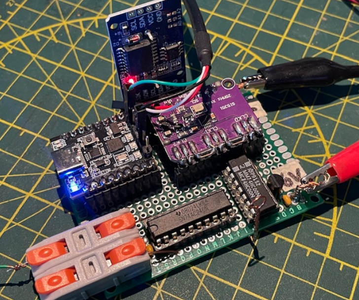
If you pick up my WSPR beacon on 80m, this is what the signal came from: a homebrew built-from-first-principles design. The oscillator is a 74HC00 NAND gate. The NTSC color burst crystal was modified with a Sharpie to oscillate on 3570.1 kHz.
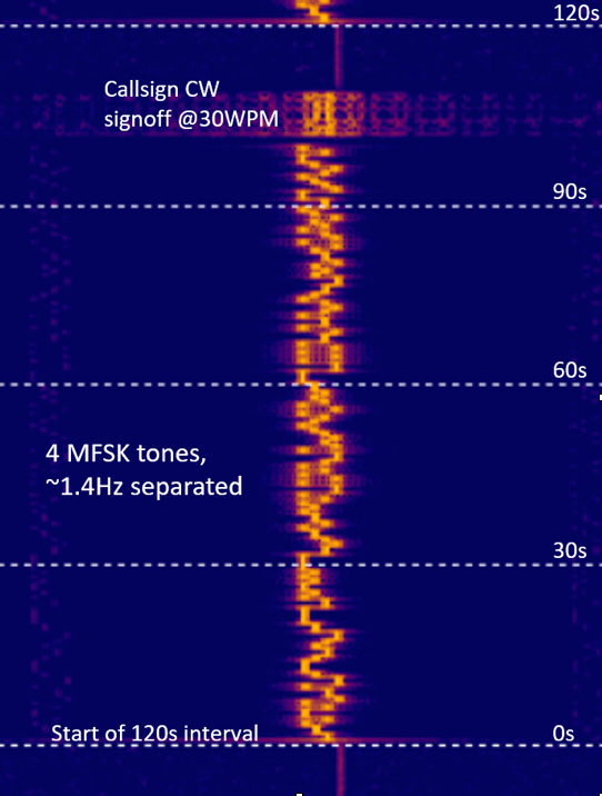
A second NAND gate is used to gate the oscillator signal, producing CW. I sign off my WSPR transmissions with my callsign in CW.
The microcontroller is an ATTiny88 in some Arduino form factor. I never developed an interest in object-oriented programming, so I usually wipe the bootloader and write my own code in assembler or sometimes a higher-level language.
Time comes from a DS3121 RTC. Drift is deep sub-second per day, but it needs occasional tuning to keep the drift under a second.
WSPR modulation is created by driving a low-pass-filtered PWM signal into a reverse-biased red LED, which is used as a varactor in the crystal circuit. A few pF is enough to pull the crystal over the ~4.5Hz range dictated by the WSPR protocol.
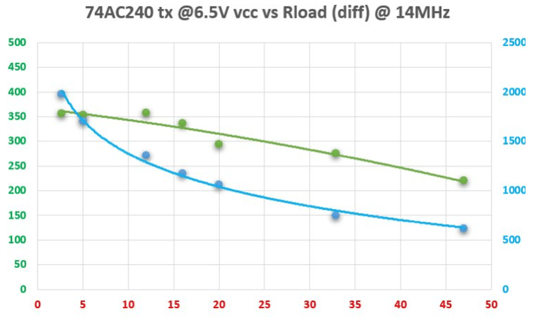
The PA is a 74AC240 with two times 4 drivers driven differentially. I measured the differential output impedance to be about 17 ohms, so I use a 5:1 balanced-to-balanced impedance transformer (a balbal?), giving about 90 ohms to the antenna port. LPF is a 5th-order differential Butterworth LC filter. I know I should not have used an SMA connector, but I was originally not planning on a differential drive.
Power is a single Li-Ion cell, with no power conversion. This causes about 20Hz of drift over the supply range. The 2Ah cell powers the beacon through the night.
The transmission line to the antenna is about 30m / 100ft of Cat-5 network cable.
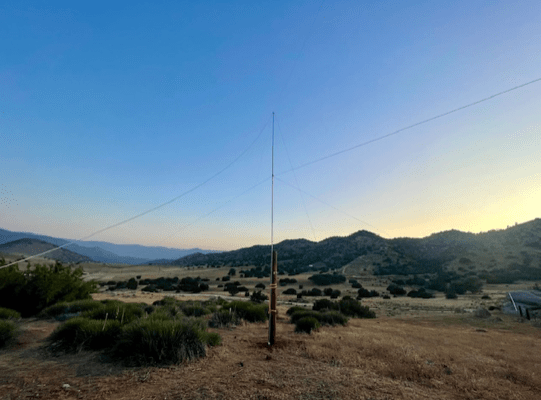
The antenna is an inverted V with the apex at 30ft / 10m, but unfortunately, 100mW will not boil off any clouds.
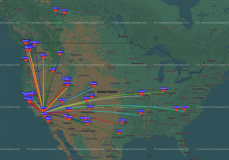
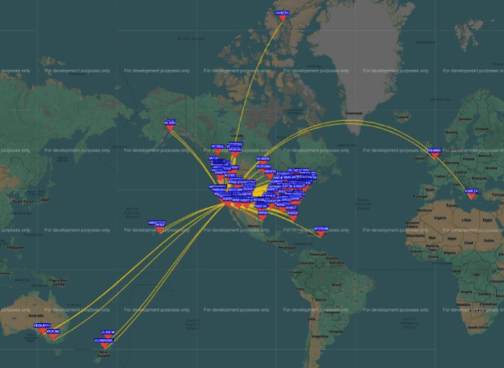
One night of operation on one battery charge yields the following. I’m rather pleased with that for 100mW of power into an inverted V at one-eighth of a wavelength high.
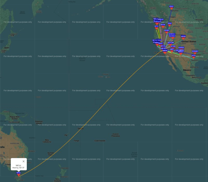
It was even spotted in Tasmania — with 100 mW, on 80m! On a couple of occasions, it got to Alaska, which I thought was pretty good, but Exceter in Tasmania is 12,839km. Almost 130,000 km per watt, with an NVIS antenna made from garbage wire (24 Ga CCA, so aluminum).
If you pick up my WSPR beacon on 20m, the story is somewhat different. This is a more “traditional” approach, using an Si5351A CMOS clock generator programmed around the 20m WSPR frequencies on both sides of 14.097100 MHz.
The rest is mostly the same; the LVDS 3.3V p-p signal is boosted to 5V with a 74HC gate, and the PA is a 74AC240, here driven at 6V.
When loaded between 15 and 20 ohms differentially, Pout is around 300mW, and PA dissipation is about a Watt before the output filter. The transmission line (CAT-5) is over 20 ohms resistively alone. The ERP is about 100mW into a resonant inverted V about 7 meters up. 20m is an easy band, so down under and “up over” at VY0ERC showed up within hours.
Our mission at ClearSkyRF is to provide a low-threshold experimental environment that unleashes new forms of creativity and scientific insight.
Using what’s at hand and making the most of your surroundings is critical to gaining quick insights without the high price tag associated with formal experimentation.
In this series, I share documentation from my past experiments — hopefully to spark ideas and conversations.
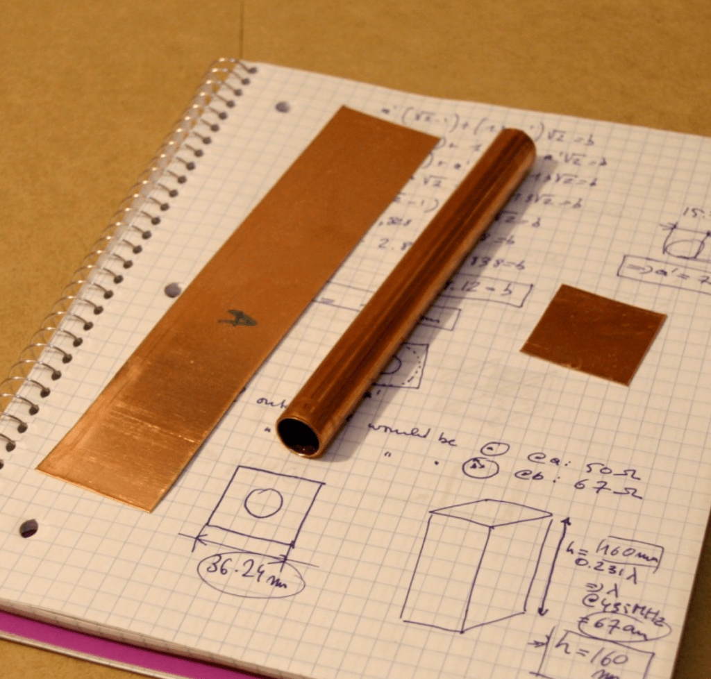
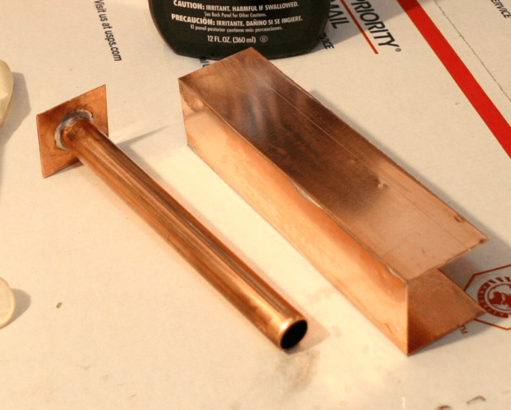
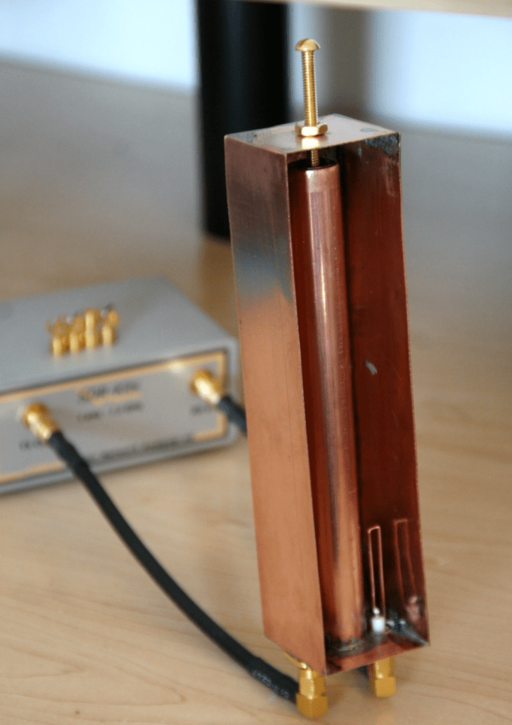
First up, here’s a cavity filter for 70cm wavelength: